
 免费 AI IDE

距离变换的图像分割和Watershed算法
2018-09-28 11:29 更新
目标
在本教程中,您将学习如何:
- 使用OpenCV函数cv :: filter2D为了执行一些拉普拉斯滤波来进行图像锐化
- 使用OpenCV函数cv :: distanceTransform来获得二进制图像的导出表示,其中每个像素的值被替换为最近的背景像素的距离
- 使用OpenCV函数cv :: watershed来隔离图像中的对象与背景
Code
本教程代码如下所示。您也可以从这里下载。
#include <opencv2/opencv.hpp>
#include <iostream>
using namespace std;
using namespace cv;
int main()
{
    // Load the image
    Mat src = imread("../data/cards.png");
    // Check if everything was fine
    if (!src.data)
        return -1;
    // Show source image
    imshow("Source Image", src);
    // Change the background from white to black, since that will help later to extract
    // better results during the use of Distance Transform
    for( int x = 0; x < src.rows; x++ ) {
      for( int y = 0; y < src.cols; y++ ) {
          if ( src.at<Vec3b>(x, y) == Vec3b(255,255,255) ) {
            src.at<Vec3b>(x, y)[0] = 0;
            src.at<Vec3b>(x, y)[1] = 0;
            src.at<Vec3b>(x, y)[2] = 0;
          }
        }
    }
    // Show output image
    imshow("Black Background Image", src);
    // Create a kernel that we will use for accuting/sharpening our image
    Mat kernel = (Mat_<float>(3,3) <<
            1,  1, 1,
            1, -8, 1,
            1,  1, 1); // an approximation of second derivative, a quite strong kernel
    // do the laplacian filtering as it is
    // well, we need to convert everything in something more deeper then CV_8U
    // because the kernel has some negative values,
    // and we can expect in general to have a Laplacian image with negative values
    // BUT a 8bits unsigned int (the one we are working with) can contain values from 0 to 255
    // so the possible negative number will be truncated
    Mat imgLaplacian;
    Mat sharp = src; // copy source image to another temporary one
    filter2D(sharp, imgLaplacian, CV_32F, kernel);
    src.convertTo(sharp, CV_32F);
    Mat imgResult = sharp - imgLaplacian;
    // convert back to 8bits gray scale
    imgResult.convertTo(imgResult, CV_8UC3);
    imgLaplacian.convertTo(imgLaplacian, CV_8UC3);
    // imshow( "Laplace Filtered Image", imgLaplacian );
    imshow( "New Sharped Image", imgResult );
    src = imgResult; // copy back
    // Create binary image from source image
    Mat bw;
    cvtColor(src, bw, CV_BGR2GRAY);
    threshold(bw, bw, 40, 255, CV_THRESH_BINARY | CV_THRESH_OTSU);
    imshow("Binary Image", bw);
    // Perform the distance transform algorithm
    Mat dist;
    distanceTransform(bw, dist, CV_DIST_L2, 3);
    // Normalize the distance image for range = {0.0, 1.0}
    // so we can visualize and threshold it
    normalize(dist, dist, 0, 1., NORM_MINMAX);
    imshow("Distance Transform Image", dist);
    // Threshold to obtain the peaks
    // This will be the markers for the foreground objects
    threshold(dist, dist, .4, 1., CV_THRESH_BINARY);
    // Dilate a bit the dist image
    Mat kernel1 = Mat::ones(3, 3, CV_8UC1);
    dilate(dist, dist, kernel1);
    imshow("Peaks", dist);
    // Create the CV_8U version of the distance image
    // It is needed for findContours()
    Mat dist_8u;
    dist.convertTo(dist_8u, CV_8U);
    // Find total markers
    vector<vector<Point> > contours;
    findContours(dist_8u, contours, CV_RETR_EXTERNAL, CV_CHAIN_APPROX_SIMPLE);
    // Create the marker image for the watershed algorithm
    Mat markers = Mat::zeros(dist.size(), CV_32SC1);
    // Draw the foreground markers
    for (size_t i = 0; i < contours.size(); i++)
        drawContours(markers, contours, static_cast<int>(i), Scalar::all(static_cast<int>(i)+1), -1);
    // Draw the background marker
    circle(markers, Point(5,5), 3, CV_RGB(255,255,255), -1);
    imshow("Markers", markers*10000);
    // Perform the watershed algorithm
    watershed(src, markers);
    Mat mark = Mat::zeros(markers.size(), CV_8UC1);
    markers.convertTo(mark, CV_8UC1);
    bitwise_not(mark, mark);
//    imshow("Markers_v2", mark); // uncomment this if you want to see how the mark
                                  // image looks like at that point
    // Generate random colors
    vector<Vec3b> colors;
    for (size_t i = 0; i < contours.size(); i++)
    {
        int b = theRNG().uniform(0, 255);
        int g = theRNG().uniform(0, 255);
        int r = theRNG().uniform(0, 255);
        colors.push_back(Vec3b((uchar)b, (uchar)g, (uchar)r));
    }
    // Create the result image
    Mat dst = Mat::zeros(markers.size(), CV_8UC3);
    // Fill labeled objects with random colors
    for (int i = 0; i < markers.rows; i++)
    {
        for (int j = 0; j < markers.cols; j++)
        {
            int index = markers.at<int>(i,j);
            if (index > 0 && index <= static_cast<int>(contours.size()))
                dst.at<Vec3b>(i,j) = colors[index-1];
            else
                dst.at<Vec3b>(i,j) = Vec3b(0,0,0);
        }
    }
    // Visualize the final image
    imshow("Final Result", dst);
    waitKey(0);
    return 0;
}
说明/结果
- 加载源图像并检查是否加载没有任何问题,然后显示:
    // Load the image
    Mat src = imread("../data/cards.png");
    // Check if everything was fine
    if (!src.data)
        return -1;
    // Show source image
    imshow("Source Image", src);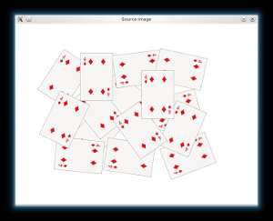
- 那么如果我们有一个有白色背景的图像,那么将它变成黑色是很好的。这将有助于我们在应用距离变换时更容易地描绘前景对象:
    // Change the background from white to black, since that will help later to extract
    // better results during the use of Distance Transform
    for( int x = 0; x < src.rows; x++ ) {
      for( int y = 0; y < src.cols; y++ ) {
          if ( src.at<Vec3b>(x, y) == Vec3b(255,255,255) ) {
            src.at<Vec3b>(x, y)[0] = 0;
            src.at<Vec3b>(x, y)[1] = 0;
            src.at<Vec3b>(x, y)[2] = 0;
          }
        }
    }
    // Show output image
    imshow("Black Background Image", src);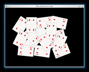
- 之后,我们将锐化我们的形象,以锐化前景对象的边缘。我们将应用一个具有相当强的滤波器的拉普拉斯滤波器(二阶导数近似):
    // Create a kernel that we will use for accuting/sharpening our image
    Mat kernel = (Mat_<float>(3,3) <<
            1,  1, 1,
            1, -8, 1,
            1,  1, 1); // an approximation of second derivative, a quite strong kernel
    // do the laplacian filtering as it is
    // well, we need to convert everything in something more deeper then CV_8U
    // because the kernel has some negative values,
    // and we can expect in general to have a Laplacian image with negative values
    // BUT a 8bits unsigned int (the one we are working with) can contain values from 0 to 255
    // so the possible negative number will be truncated
    Mat imgLaplacian;
    Mat sharp = src; // copy source image to another temporary one
    filter2D(sharp, imgLaplacian, CV_32F, kernel);
    src.convertTo(sharp, CV_32F);
    Mat imgResult = sharp - imgLaplacian;
    // convert back to 8bits gray scale
    imgResult.convertTo(imgResult, CV_8UC3);
    imgLaplacian.convertTo(imgLaplacian, CV_8UC3);
    // imshow( "Laplace Filtered Image", imgLaplacian );
    imshow( "New Sharped Image", imgResult );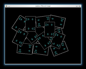

- 现在我们分别从我们的新锐的源图像转换为灰度和二进制图像:
    // Create binary image from source image
    Mat bw;
    cvtColor(src, bw, CV_BGR2GRAY);
    threshold(bw, bw, 40, 255, CV_THRESH_BINARY | CV_THRESH_OTSU);
    imshow("Binary Image", bw);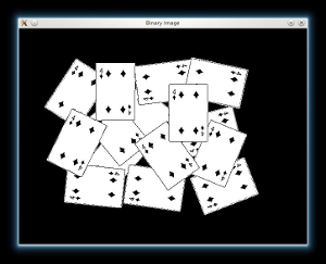
- 我们准备好在二进制图像上应用Distance Tranform。此外,我们规范化输出图像,以便能够可视化和阈值结果:
    // Perform the distance transform algorithm
    Mat dist;
    distanceTransform(bw, dist, CV_DIST_L2, 3);
    // Normalize the distance image for range = {0.0, 1.0}
    // so we can visualize and threshold it
    normalize(dist, dist, 0, 1., NORM_MINMAX);
    imshow("Distance Transform Image", dist);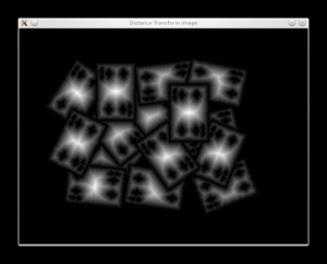
- 我们阈值dist图像,然后执行一些形态学操作(即扩张),以从上述图像中提取峰值:
    // Threshold to obtain the peaks
    // This will be the markers for the foreground objects
    threshold(dist, dist, .4, 1., CV_THRESH_BINARY);
    // Dilate a bit the dist image
    Mat kernel1 = Mat::ones(3, 3, CV_8UC1);
    dilate(dist, dist, kernel1);
    imshow("Peaks", dist);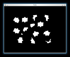
- 从每个blob,然后我们在cv :: findContours函数的帮助下创建一个watershed算法的种子/标记:
    // Create the CV_8U version of the distance image
    // It is needed for findContours()
    Mat dist_8u;
    dist.convertTo(dist_8u, CV_8U);
    // Find total markers
    vector<vector<Point> > contours;
    findContours(dist_8u, contours, CV_RETR_EXTERNAL, CV_CHAIN_APPROX_SIMPLE);
    // Create the marker image for the watershed algorithm
    Mat markers = Mat::zeros(dist.size(), CV_32SC1);
    // Draw the foreground markers
    for (size_t i = 0; i < contours.size(); i++)
        drawContours(markers, contours, static_cast<int>(i), Scalar::all(static_cast<int>(i)+1), -1);
    // Draw the background marker
    circle(markers, Point(5,5), 3, CV_RGB(255,255,255), -1);
    imshow("Markers", markers*10000);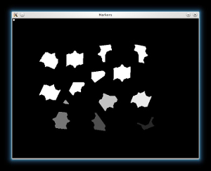
- 最后,我们可以应用watershed算法,并可视化结果:
    // Perform the watershed algorithm
    watershed(src, markers);
    Mat mark = Mat::zeros(markers.size(), CV_8UC1);
    markers.convertTo(mark, CV_8UC1);
    bitwise_not(mark, mark);
//    imshow("Markers_v2", mark); // uncomment this if you want to see how the mark
                                  // image looks like at that point
    // Generate random colors
    vector<Vec3b> colors;
    for (size_t i = 0; i < contours.size(); i++)
    {
        int b = theRNG().uniform(0, 255);
        int g = theRNG().uniform(0, 255);
        int r = theRNG().uniform(0, 255);
        colors.push_back(Vec3b((uchar)b, (uchar)g, (uchar)r));
    }
    // Create the result image
    Mat dst = Mat::zeros(markers.size(), CV_8UC3);
    // Fill labeled objects with random colors
    for (int i = 0; i < markers.rows; i++)
    {
        for (int j = 0; j < markers.cols; j++)
        {
            int index = markers.at<int>(i,j);
            if (index > 0 && index <= static_cast<int>(contours.size()))
                dst.at<Vec3b>(i,j) = colors[index-1];
            else
                dst.at<Vec3b>(i,j) = Vec3b(0,0,0);
        }
    }
    // Visualize the final image
    imshow("Final Result", dst);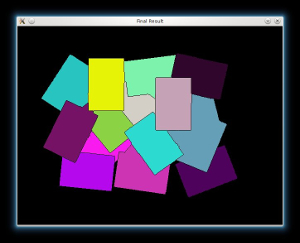
以上内容是否对您有帮助:


更多建议: