Example: Train error vs Test error

Train error vs Test error

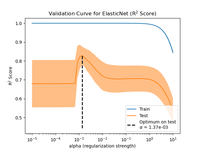
Illustration of how the performance of an estimator on unseen data (test data) is not the same as the performance on training data. As the regularization increases the performance on train decreases while the performance on test is optimal within a range of values of the regularization parameter. The example with an Elastic-Net regression model and the performance is measured using the explained variance a.k.a. R^2.

print(__doc__)

# Author: Alexandre Gramfort <alexandre.gramfort@inria.fr>
# License: BSD 3 clause

import numpy as np
from sklearn import linear_model

Generate sample data

n_samples_train, n_samples_test, n_features = 75, 150, 500
np.random.seed(0)
coef = np.random.randn(n_features)
coef[50:] = 0.0  # only the top 10 features are impacting the model
X = np.random.randn(n_samples_train + n_samples_test, n_features)
y = np.dot(X, coef)

# Split train and test data
X_train, X_test = X[:n_samples_train], X[n_samples_train:]
y_train, y_test = y[:n_samples_train], y[n_samples_train:]

Compute train and test errors

alphas = np.logspace(-5, 1, 60)
enet = linear_model.ElasticNet(l1_ratio=0.7)
train_errors = list()
test_errors = list()
for alpha in alphas:
    enet.set_params(alpha=alpha)
    enet.fit(X_train, y_train)
    train_errors.append(enet.score(X_train, y_train))
    test_errors.append(enet.score(X_test, y_test))

i_alpha_optim = np.argmax(test_errors)
alpha_optim = alphas[i_alpha_optim]
print("Optimal regularization parameter : %s" % alpha_optim)

# Estimate the coef_ on full data with optimal regularization parameter
enet.set_params(alpha=alpha_optim)
coef_ = enet.fit(X, y).coef_

Out:

Optimal regularization parameter : 0.000335292414925

Plot results functions

import matplotlib.pyplot as plt
plt.subplot(2, 1, 1)
plt.semilogx(alphas, train_errors, label='Train')
plt.semilogx(alphas, test_errors, label='Test')
plt.vlines(alpha_optim, plt.ylim()[0], np.max(test_errors), color='k',
           linewidth=3, label='Optimum on test')
plt.legend(loc='lower left')
plt.ylim([0, 1.2])
plt.xlabel('Regularization parameter')
plt.ylabel('Performance')

# Show estimated coef_ vs true coef
plt.subplot(2, 1, 2)
plt.plot(coef, label='True coef')
plt.plot(coef_, label='Estimated coef')
plt.legend()
plt.subplots_adjust(0.09, 0.04, 0.94, 0.94, 0.26, 0.26)
plt.show()

Total running time of the script: (0 minutes 2.684 seconds)