Example: Automatic Relevance Determination Regression

Automatic Relevance Determination Regression (ARD)

Fit regression model with Bayesian Ridge Regression.

See Bayesian Ridge Regression for more information on the regressor.

Compared to the OLS (ordinary least squares) estimator, the coefficient weights are slightly shifted toward zeros, which stabilises them.

The histogram of the estimated weights is very peaked, as a sparsity-inducing prior is implied on the weights.

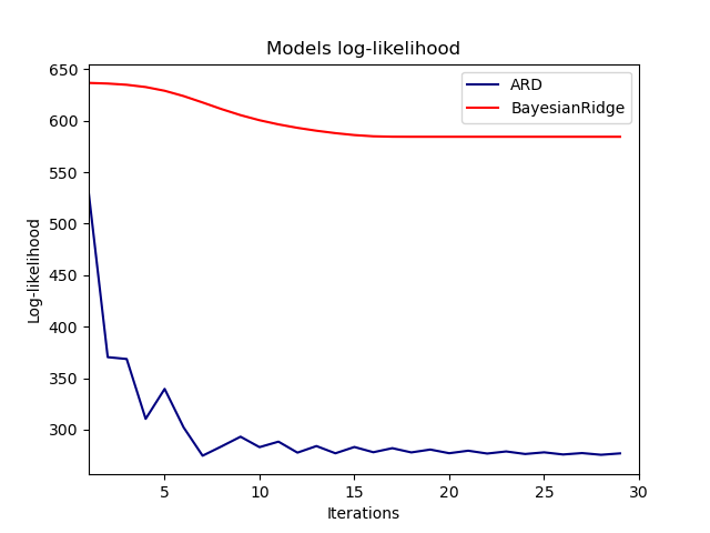
The estimation of the model is done by iteratively maximizing the marginal log-likelihood of the observations.

print(__doc__)

import numpy as np
import matplotlib.pyplot as plt
from scipy import stats

from sklearn.linear_model import ARDRegression, LinearRegression

Generating simulated data with Gaussian weights

# Parameters of the example
np.random.seed(0)
n_samples, n_features = 100, 100
# Create Gaussian data
X = np.random.randn(n_samples, n_features)
# Create weights with a precision lambda_ of 4.
lambda_ = 4.
w = np.zeros(n_features)
# Only keep 10 weights of interest
relevant_features = np.random.randint(0, n_features, 10)
for i in relevant_features:
    w[i] = stats.norm.rvs(loc=0, scale=1. / np.sqrt(lambda_))
# Create noise with a precision alpha of 50.
alpha_ = 50.
noise = stats.norm.rvs(loc=0, scale=1. / np.sqrt(alpha_), size=n_samples)
# Create the target
y = np.dot(X, w) + noise

Fit the ARD Regression

clf = ARDRegression(compute_score=True)
clf.fit(X, y)

ols = LinearRegression()
ols.fit(X, y)

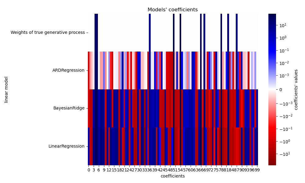
Plot the true weights, the estimated weights and the histogram of the weights

plt.figure(figsize=(6, 5))
plt.title("Weights of the model")
plt.plot(clf.coef_, color='darkblue', linestyle='-', linewidth=2,
         label="ARD estimate")
plt.plot(ols.coef_, color='yellowgreen', linestyle=':', linewidth=2,
         label="OLS estimate")
plt.plot(w, color='orange', linestyle='-', linewidth=2, label="Ground truth")
plt.xlabel("Features")
plt.ylabel("Values of the weights")
plt.legend(loc=1)

plt.figure(figsize=(6, 5))
plt.title("Histogram of the weights")
plt.hist(clf.coef_, bins=n_features, color='navy', log=True)
plt.scatter(clf.coef_[relevant_features], 5 * np.ones(len(relevant_features)),
            color='gold', marker='o', label="Relevant features")
plt.ylabel("Features")
plt.xlabel("Values of the weights")
plt.legend(loc=1)

plt.figure(figsize=(6, 5))
plt.title("Marginal log-likelihood")
plt.plot(clf.scores_, color='navy', linewidth=2)
plt.ylabel("Score")
plt.xlabel("Iterations")
plt.show()

Total running time of the script: (0 minutes 0.443 seconds)