Querying or Reading Data

Querying or Reading Data

OpenTSDB offers a number of means to extract data such as CLI tools, an HTTP API and as a GnuPlot graph. Querying with OpenTSDB's tag based system can be a bit tricky so read through this document and checkout the following pages for deeper information. Example queries on this page follow the HTTP API format.

Query Components

OpenTSDB's query language is fairly simple but flexible. Each query has the following components:

Parameter	Date Type	Required	Description	Example
Start Time	String or Integer	Yes	Starting time for the query. This may be an absolute or relative time. See Dates and Times for details	24h-ago
End Time	String or Integer	No	An end time for the query. If the end time is not supplied, the current time on the TSD will be used. See Dates and Times for details.	1h-ago
Metric	String	Yes	The full name of a metric in the system. Must be the complete name. Case sensitive	sys.cpu.user
Aggregation Function	String	Yes	A mathematical function to use in combining multiple time series	sum
Tags	String	No	An optional set of tags for filtering or grouping	host=*,dc=lax
Downsampler	String	No	An optional interval and function to reduce the number of data points returned	1h-avg
Rate	String	No	An optional flag to calculate the rate of change for the result	rate

Times

Absolute time stamps are supported in human readable format or Unix style integers. Relative times may be used for refreshing dashboards. Currently, all queries are able to cover a single time span. In the future we hope to provide an offset query parameter that would allow for aggregations or graphing of a metric over different time periods, such as comparing last week to 1 year ago. See Dates and Times for details on what is permissible.

While OpenTSDB can store data with millisecond resolution, most queries will return the data with second resolution to provide backwards compatibility for existing tools. Unless a down sampling algorithm has been specified with a query, the data will automatically be down sampled to 1 second using the same aggregation function specified in a query. This way, if multiple data points are stored for a given second, they will be aggregated and returned in a normal query correctly.

To extract data with millisecond resolution, use the /api/query endpoint and specify the msResolution (ms` is also okay, but not recommended) JSON parameter or query string flag and it will bypass down sampling (unless specified) and return all timestamps in Unix epoch millisecond resolution. Also, the scan commandline utility will return the timestamp as written in storage.

Tags

Every time series is comprised of a metric and one or more tag name/value pairs. Since tags are optional in queries, if you request only the metric name, then every metric with any number or value of tags will be returned in the aggregated results. For example, if we have a stored data set:

sys.cpu.user host=webserver01,cpu=0  1356998400  1
sys.cpu.user host=webserver01,cpu=1  1356998400  4
sys.cpu.user host=webserver02,cpu=0  1356998400  2
sys.cpu.user host=webserver02,cpu=1  1356998400  1

and simply craft a query start=1356998400&m=sum:sys.cpu.user, we will get a value of 8 at 1356998400 that incorporates all 4 time series.

If we want to aggregate the results for a specific group, we can filter on the host tag. The query start=1356998400&m=sum:sys.cpu.user{host=webserver01} will return a value of 5, incorporating only the time series where host=webserver01. To drill down to a specific time series, you must include all of the tags for the series, e.g. start=1356998400&m=sum:sys.cpu.user{host=webserver01,cpu=0} will return 1.

Grouping

A query can also aggregate time series with multiple tags into groups based on a tag value. Two special characters can be passed to the right of the equals symbol in a query:

• * - The asterisk will return a separate result for each unique tag value
• | - The pipe will return a separate result only for the exact tag values specified

Let's take the following data set as an example:

sys.cpu.user host=webserver01,cpu=0  1356998400  1
sys.cpu.user host=webserver01,cpu=1  1356998400  4
sys.cpu.user host=webserver02,cpu=0  1356998400  2
sys.cpu.user host=webserver02,cpu=1  1356998400  1
sys.cpu.user host=webserver03,cpu=0  1356998400  5
sys.cpu.user host=webserver03,cpu=1  1356998400  3

If we want to query for the average CPU time across each server we can craft a query like start=1356998400&m=avg:sys.cpu.user{host=*}. This will give us three results:

1. The aggregated average for sys.cpu.user host=webserver01,cpu=0 and sys.cpu.user host=webserver01,cpu=1
2. The aggregated average for sys.cpu.user host=webserver02,cpu=0 and sys.cpu.user host=webserver02,cpu=1
3. The aggregated average for sys.cpu.user host=webserver03,cpu=0 and sys.cpu.user host=webserver03,cpu=1

However if we have many web servers in the system, this could create a ton of results. To filter on only the hosts we want you can use the pipe operator to select a subset of time series. For example start=1356998400&m=avg:sys.cpu.user{host=webserver01|webserver03} will return results only for webserver01 and webserver03.

With version 2.2 you can enable or disable grouping per tag filter. Additional filters are also available including wildcards and regular expressions.

Explicit Tags

As of 2.3 and later, if you know all of the tag keys for a given metric query latency can be improved greatly by using the explicitTags feature and making sure tsd.query.enable_fuzzy_filter is enabled in the config. A special filter is given to HBase that enables skipping ahead to rows that we need for the query instead of iterating over every row key and comparing a regular expression.

For example, using the data set above, if we only care about metrics where host=webserver02 and there are hundreds of hosts, you can craft a query such as start=1356998400&m=avg:explicit_tags:sys.cpu.user{host=webserver02,cpu=*}. Note that you must specify every tag included in the time series for this to work and you can decide whether or not to group by the additional tags.

Aggregation

A powerful feature of OpenTSDB is the ability to perform on-the-fly aggregations of multiple time series into a single set of data points. The original data is always available in storage but we can quickly extract the data in meaningful ways. Aggregation functions are means of merging two or more data points for a single time stamp into a single value. See Aggregators for details.

Interpolation

When performing an aggregation, what happens if the time stamps of the data points for each time series fail to line up? Say we record the temperature every 5 minutes in different regions around the world. A sensor in Paris may send a temperature of 27c at 1356998400. Then a sensor in San Francisco may send a value of 18c at 1356998430, 30 seconds later. Antarctica may report -29c at 1356998529. If we run a query requesting the average temperature, we want all of the data points averaged together into a single point. This is where interpolation comes into play. See Aggregators for details.

Downsampling

OpenTSDB can ingest a large amount of data, even a data point every second for a given time series. Thus queries may return a large number of data points. Accessing the results of a query with a large number of points from the API can eat up bandwidth. High frequencies of data can easily overwhelm Javascript graphing libraries, hence the choice to use GnuPlot. Graphs created by the GUI can be difficult to read, resulting in thick lines such as the graph below:

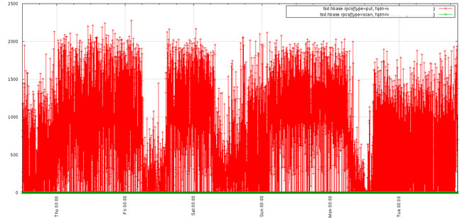
Down sampling can be used at query time to reduce the number of data points returned so that you can extract better information from a graph or pass less data over a connection. Down sampling requires an aggregation function and a time interval. The aggregation function is used to compute a new data point across all of the data points in the specified interval with the proper mathematical function. For example, if the aggregation sum is used, then all of the data points within the interval will be summed together into a single value. If avg is chosen, then the average of all data points within the interval will be returned.

Intervals are specified by a number and a unit of time. For example, 30m will aggregate data points every 30 minutes. 1h will aggregate across an hour. See Dates and Times for valid relative time units. Do not add the -ago to a down sampling query.

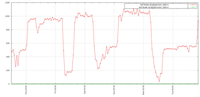
Using down sampling we can cleanup the previous graph to arrive at something much more useful:

As of 2.1, downsampled timestamps are normalized based on the remainder of the original data point timestamp divided by the downsampling interval in milliseconds, i.e. the modulus. In Java the code is timestamp - (timestamp % interval_ms). For example, given a timestamp of 1388550980000, or 1/1/2014 04:36:20 UTC and an hourly interval that equates to 3600000 milliseconds, the resulting timestamp will be rounded to 1388548800000. All data points between 4 and 5 UTC will wind up in the 4 AM bucket. If you query for a day's worth of data downsampling on 1 hour, you will receive 24 data points (assuming there is data for all 24 hours).

Normalization works very well for common queries such as a day's worth of data downsampled to 1 minute or 1 hour. However if you try to downsample on an odd interval, such as 36 minutes, then the timestamps may look a little strange due to the nature of the modulus calculation. Given an interval of 36 minutes and our example above, the interval would be 2160000 milliseconds and the resulting timestamp 1388549520 or 04:12:00 UTC. All data points between 04:12 and 04:48 would wind up in a single bucket. Also note that OpenTSDB cannot currently normalize on non-UTC times and it cannot normalize on weekly or monthly boundaries.

With version 2.2 a downsampling query can emit a NaN or null when a downsample bucket is missing a value for all of the series involved. Because OpenTSDB does not allow for storing literal NaNs at this time, nor does it impose specific intervals on storage, this can be used to mimic systems that do such as RRDs.

Rate

A number of data sources return values as constantly incrementing counters. One example is a web site hit counter. When you start a web server, it may have a hit counter of 0. After five minutes the value may be 1,024. After another five minutes it may be 2,048. The graph for a counter will be a somewhat straight line angling up to the right and isn't always very useful. OpenTSDB provides the rate key word that calculates the rate of change in values over time. This will transform counters into lines with spikes to show you when activity occurred and can be much more useful.

The rate is the first derivative of the values. It's defined as (v2 - v1) / (t2 - t1). Therefore you will get the rate of change per second. Currently the rate of change between millisecond values defaults to a per second calculation.

OpenTSDB 2.0 provides support for special monotonically increasing counter data handling including the ability to set a "rollover" value and suppress anomalous fluctuations. When the counterMax value is specified in a query, if a data point approaches this value and the point after is less than the previous, the max value will be used to calculate an accurate rate given the two points. For example, if we were recording an integer counter on 2 bytes, the maximum value would be 65,535. If the value at t0 is 64000 and the value at t1 is 1000, the resulting rate per second would be calculated as -63000. However we know that it's likely the counter rolled over so we can set the max to 65535 and now the calculation will be 65535 - t0 + t1 to give us 2535.

Systems that track data in counters often revert to 0 when restarted. When that happens and we could get a spurious result when using the max counter feature. For example, if the counter has reached 2000 at t0 and someone reboots the server, the next value may be 500 at t1. If we set our max to 65535 the result would be 65535 - 2000 + 500 to give us 64035. If the normal rate is a few points per second, this particular spike, with 30s between points, would create a rate spike of 2,134.5! To avoid this, we can set the resetValue which will, when the rate exceeds this value, return a data point of 0 so as to avoid spikes in either direction. For the example above, if we know that our rate almost never exceeds 100, we could configure a resetValue of 100 and when the data point above is calculated, it will return 0 instead of 2,134.5. The default value of 0 means the reset value will be ignored, no rates will be suppressed.

Order of operations

Understanding the order of operations is important. When returning query results the following is the order in which processing takes place:

1. Grouping
2. Down Sampling
3. Interpolation
4. Aggregation
5. Rate Calculation